Longitudinal Data Analysis

Metaviz is a tool for interactive visualization and exploration of metagenomic sequencing data. It provides a novel navigation tool for exploring hierarchical feature data that is coupled with multiple data visualizations including heatmaps, stacked bar charts, and scatter plots. The metavizr package implements two-way communication between the R/Bioconductor computational genomics environment and Metaviz. Objects in an R/Bioconductor session can be visualized and explored using the Metaviz navigation tool and plots. In this post we show how to use metavizr and the metagenomeSeq Bioconductor package to analyze data from a longitudinal study.

Generating metagenomeSeq objects and performing SS-ANOVA testing

We use a dataset from “Individual-specific changes in the human gut microbiota after challenge with enterotoxigenic Escherichia coli and subsequent ciprofloxacin treatment” which includes data from 12 human samples that were challenged with E. coli then provided subsequent antibiotic treatment.
Samples were taken for 1 day pre-infection and 10 days post-infection. We will analyze this time series data with a smoothing-spline and plot it in a Metaviz workspace with a line plot over all features.

First, import the etec16s dataset, select sample data from the first 9 days. Then use metavizr to launch an instance of the Metaviz app in a local web-browser.

library(etec16s)
library(metagenomeSeq)
library(metavizr)
data(etec16s)
etec16s <- etec16s[,-which(pData(etec16s)$Day>9)]

app <- startMetaviz("http://metaviz.cbcb.umd.edu") 

This provides a new workspace.

Next, use metagenomeSeq to fit a smoothing-spline to the time series data using the ‘timeSeriesFits’ method.

featureData(etec16s)$Kingdom <- "Bacteria"
feature_order <- c("Kingdom", "Phylum", "Class", "Order", "Family", "Genus", "Species", "OTU.ID")

timeSeriesFits <- fitMultipleTimeSeries(obj=etec16s,
                             formula = abundance~id + time*class + AntiGiven,
                             class="AnyDayDiarrhea",
                             id="SubjectID",
                             time="Day",
                             lvl="Species",
                             feature_order = feature_order,
                             C=0.3,
                             B=1)

Generating metavizR object to plot

For plotting the data using Metaviz, we use the fit values as y-coordinates and timepoints as x-coordinates. We need to call ‘ts2MRexperiment’ with arguments for the sample and feature data, in this case timepoints and annotations, respectively. We also aggregate to the ‘species’ level.

feature_order2 <- c("Kingdom", "Phylum", "Class", "Order", "Family", "Genus", "Species")

splinesMRexp <- ts2MRexperiment(timeSeriesFits, feature_data = featureData(aggregateByTaxonomy(etec16s, lvl="Species", feature_order = feature_order2)), sampleNames = timeSeriesFits[[2]]$fit$timePoints)
etec16s_species <- aggregateByTaxonomy(etec16s, lvl="Species", feature_order = feature_order)

Choosing features to plot and adding a line plot to Metaviz

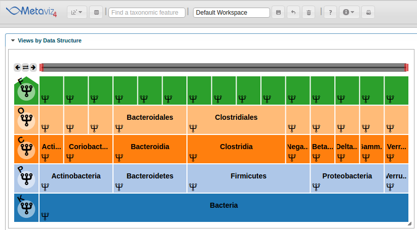
We select features with a timepoint with absolute log-fold change greater than 2. We add the MRexperiment as a measurement for Metaviz to plot the hierarchy in a ‘FacetZoom’ object.

splines_to_plot <- sapply(1:nrow(MRcounts(splinesMRexp)), function(i) {max(abs(MRcounts(splinesMRexp[i,]))) >= 2})
splines_to_plot_indices <- which(splines_to_plot == TRUE)

ic_plot <- app$plot(splinesMRexp[splines_to_plot_indices,], datasource_name = "etec16_base", control=metavizControl(norm = FALSE, aggregateAtDepth = 6), feature_order = feature_order2)

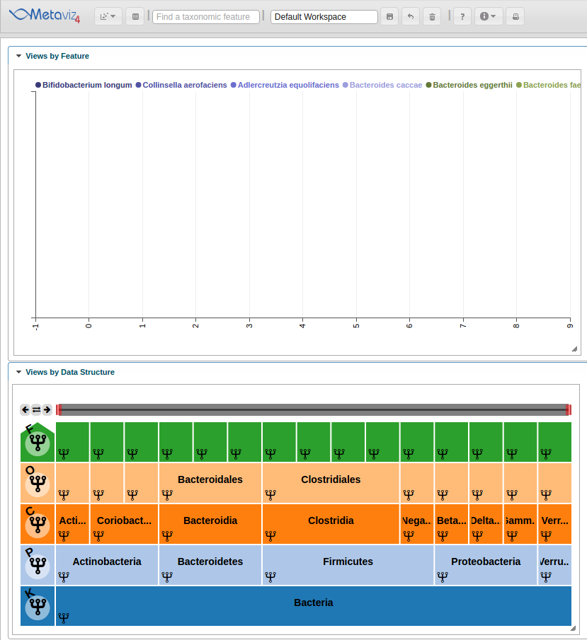
We then use the ‘revisualize’ method to add a Line Plot for the smoothing spline.

splineObj <- app$data_mgr$add_measurements(splinesMRexp[splines_to_plot_indices,], datasource_name = "etec16_base", control = metavizControl(norm=FALSE, aggregateAtDepth = 6))
splineMeasurements <- splineObj$get_measurements()
splineChart <- app$chart_mgr$visualize("LinePlot", splineMeasurements)

This adds the Line Plot to the workspace but we will need to set the range of the y-axis and modify the color scheme to produce a final workspace.

Updating chart settings from metavizR

We can update the colors and settings on the spline chart. For example, lets limit the y axis to be between -10 and 10. To do so we use the ‘set_chart_settings’ method. We can list existing settings for a chart using the ‘list_chart_settings’ function.

# list available charts
app$chart_mgr$list_chart_types()

# list available settings for "LinePlot"
app$chart_mgr$list_chart_type_settings("LinePlot")

# update settings on splineChart 
settings <- list(yMin = -10, yMax = 10)
colors <- c("#1f77b4", "#ff7f0e", "#2ca02c", "#d62728", "#9467bd", "#8c564b", "#e377c2", "#7f7f7f", "#bcbd22", "#17becf")
app$chart_mgr$set_chart_settings(splineChart, settings=settings, colors = colors)

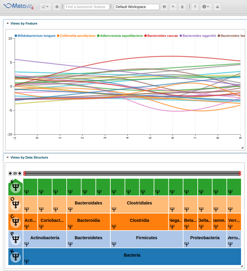
We can interact with the Metaviz session, such as hovering over the Line Plot to see highlight the path through the hierarchy.

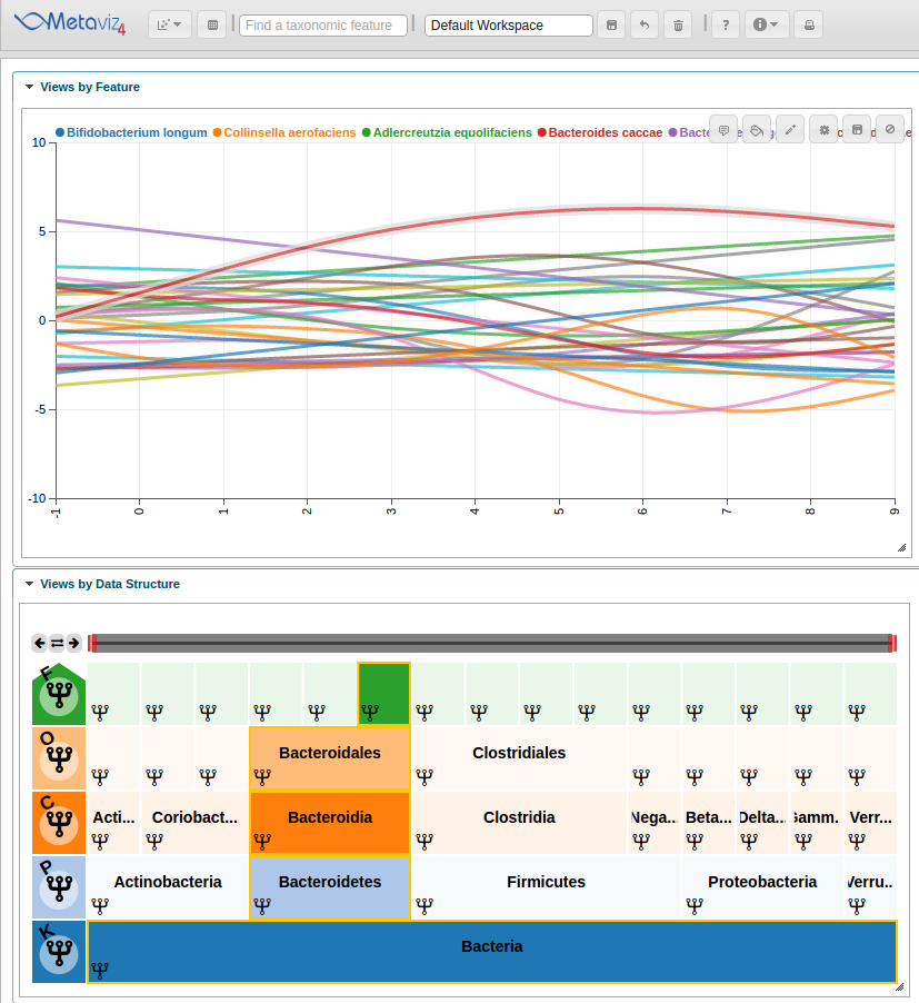
Also, we can hover in the icicle plot to highlight all features under that path in the Line Plot.