Introduction to metavizr: interactive visualization for metagenomics
Héctor Corrada Bravo, Florin Chelaru, Justin Wagner, Jayaram Kancherla, Joseph Paulson
2017-02-02
Metaviz is tool for interactive visualization and exploration of metagenomic sequencing data. Metaviz a provides main navigation tool for exploring hierarchical feature data that is coupled with multiple data visualizations including heatmaps, stacked bar charts, and scatter plots. Metaviz supports a flexible plugin framework so users can add new d3 visualizations. You can find more information about Metaviz at http://metaviz.cbcb.umd.edu/help.
The metavizr package implements two-way communication between the R/Bioconductor computational genomics environment and Metaviz. Objects in an R/Bioconductor session can be visualized and explored using the Metaviz navigation tool and plots. Metavizr uses Websockets to communicate between the browser Javascript client and the R/Bioconductor session. Websockets are the protocols underlying the popular Shiny system for authoring interactive web-based reports in R.
Preliminaries: the data
In this vignette we will look at two data sets one from a case/control study and another with a time series. We load the first data set from the msd16s Bioconductor package. This data is from the Moderate to Severe Diaherrial disease study in children from four countries: Banglash, Kenya, Mali, and the Gambia. Case and control stool samples were gathered from each country across several age ranges, 0-6 months, 6-12 months, 12-18 months, 18-24 months, and 24-60 months. An analysis of this data is described in Pop et al. [1].
require(metavizr)
require(metagenomeSeq)
require(msd16s)
The metavizr session manager
The connection to Metaviz is managed through a session manager object of class EpivizApp. We can create this object and open Metaviz using the startMetaviz function.
app <- startMetaviz()This opens a websocket connection between the interactive R session and the browser client. This will allow us to visualize data stored in the Metaviz server along with data in the interactive R session.
Windows users: In Windows platforms we need to use the service function to let the interactive R session connect to the epiviz web app and serve data requests. We then escape (using ctl-c or esc depending on your environment) to continue with the interactive R session. This is required anytime you want metavizr to serve data to the web app, for example, when interacting with the UI. (We are actively developing support for non-blocking sessions in Windows platforms).
app$server$service()For vignette purposes, we will subset the 992 msd16s samples to those 301 from Bangladesh. Also, we will aggregate the count matrix to the species level. We have found that matrix sizes with YYY elements perform well for interactive visualization with an R session using WebSockets. For larger abundance matrices, we recommend using the graph database backend available at [NEED TO ADD LINK]. Once having subset the data, we normalize count data using the metagenomeSeq::cumNorm function, choose genera that have more than 5 OTUs in the dataset and select the 10 genera with largest standard deviation of log-transformed normalized counts across samples. Set aggregation level to “class”, will find features DA at this level and then change an push those changes to an MRexperiment that is aggreagted to “species” level, and then explore the hiearchy.
feature_order <- c("superkingdom", "phylum", "class", "order", "family", "genus", "species", "OTU")
aggregated_feature_order <- feature_order[1:7]

msd16s_species <- msd16s
fData(msd16s) <- fData(msd16s)[feature_order]
fData(msd16s_species) <- fData(msd16s_species)[aggregated_feature_order]

bangladesh <- msd16s[, which(pData(msd16s)$Country == "Bangladesh")]
bangladesh_species <- msd16s_species[, which(pData(msd16s_species)$Country == "Bangladesh")]

aggregated_species <-  cumNorm(aggregateByTaxonomy(bangladesh_species, lvl="species"), p = 0.75)

aggregation_level <- "class"
aggregated_bangladesh <- aggregateByTaxonomy(bangladesh, lvl=aggregation_level)

normed_bangladesh <-  cumNorm(aggregated_bangladesh, p = 0.75)
bangladesh_sample_data <-  pData(normed_bangladesh)
mod <-  model.matrix(~1+Dysentery, data = bangladesh_sample_data)
results_bangladesh <-  fitFeatureModel(normed_bangladesh, mod)
## Warning: glm.fit: algorithm did not converge## Warning: glm.fit: fitted probabilities numerically 0 or 1 occurredlogFC_bangladesh <- MRcoefs(results_bangladesh, number = nrow(normed_bangladesh))
feature_names <- rownames(logFC_bangladesh[which(logFC_bangladesh[which(abs(logFC_bangladesh$logFC) > 2),]$adjPvalues < .05),])
fSelection <- generateSelection(feature_names =feature_names , aggregation_level = aggregation_level, selection_type =2)
control <- metavizr::metavizControl(featureSelection = fSelection)
Visualizing count data from the mouseData MRExperiment object
Now we can view the data as a heatmap calling revisualize:
heatmap <- app$chart_mgr$revisualize(chart_type = "HeatmapPlot", chart = icicle_plot)Using the same data, we can also revisualize it in a stacked plot to see the abundance of various features across samples. Since the measurements are added from creating the icicle_plot, we only need to add a stacked line plot.
stackedPlot <- app$chart_mgr$revisualize(chart_type ="StackedLinePlot", chart = icicle_plot)Finally, we can update the threshold cutoff we had for fold change, pass those modifications the icicle plot, and see the updates propogate to the heat map and stacked plot. This shows the use case of statistically-guided interactive visualizations.
feature_names2 <- rownames(logFC_bangladesh[which(logFC_bangladesh[which(abs(logFC_bangladesh$logFC) > .5),]$adjPvalues < .05),])
fSelection2 <- generateSelection(feature_names =  feature_names2, aggregation_level = aggregation_level, selection_type =2)

app$get_ms_object(icicle_plot)$featureSelection(featureNames=fSelection2$featureNames, featureOrder=fSelection2$featureOrder, featureLevel=fSelection2$featureLevel, selectionType=fSelection2$selectionType)
Longitudinal Data Analysis
Another feature of metavizr is to visualize data using a line plot. We detail the steps to perform this analysis and create a line plot using Metaviz such as those used in Paulson et al. when analyzing this time series data with a smoothing-spline [2] and [3].
First, import the etec16s dataset, select sample data from the first 9 days, and choose the feature annotations of interest.
library(etec16s)
data(etec16s)
etec16s <- etec16s[,-which(pData(etec16s)$Day>9)]
featuresOfInterest <- c('Escherichia/Shigella','Faecalibacterium prausnitzii')
Next, use metagenomeSeq to fit a smoothing-spline to the time series data.
featureData(etec16s)$Kingdom <- "Bacteria"
feature_order <- c("Kingdom", "Phylum", "Class", "Order", "Family", "Genus", "Species", "OTU.ID")

timeSeriesFits <- fitMultipleTimeSeries(obj=etec16s,
                             formula = abundance~id + time*class + AntiGiven,
                             class="AnyDayDiarrhea",
                             id="SubjectID",
                             time="Day",
                             lvl="Species",
                             feature_order = feature_order,
                             C=0.3,
                             B=1)
## Warning in mspreg1(s, r, id.basis, y, wt, method, alpha, varht, random, :
## gss warning in ssanova: iteration for model selection fails to converge
## Warning in mspreg1(s, r, id.basis, y, wt, method, alpha, varht, random, :
## gss warning in ssanova: iteration for model selection fails to convergeFor plotting the data using Metaviz, we set the fit values as y-coordinates and timepoints as x-coordinates. We need to call toMRexperiment with arguments for the sample and feature data, in this case timepoints and annotations, respectively.
feature_order2 <- c("Kingdom", "Phylum", "Class", "Order", "Family", "Genus", "Species")

splinesMRexp <- ts2MRexperiment(timeSeriesFits, feature_data = featureData(aggregateByTaxonomy(etec16s, lvl="Species", feature_order = feature_order2)), sampleNames = timeSeriesFits[[2]]$fit$timePoints)
## [1] 1 2 3 4 5 6 7 8 9 10 11 12 13 14 15 16 17
## [18] 18 19 20 21 22 23 24 25 26 27 28 29 30 31 32 33 34
## [35] 35 36 37 38 39 40 41 42 43 44 45 46 47 48 49 50 51
## [52] 52 53 54 55 0 57 58 59 60 61 62 63 64 65 66 67 68
## [69] 69 70 71 72 73 74 75 0 77 78 79 80 81 82 83 84 85
## [86] 86 87 88 89 90 91 92 93 94 95 0 0 98 99 100 101 102
## [103] 103 104 105 106 107 0 0 110 111 112 113 114 115 116 117 118 119
## [120] 120 121 122 123 124 0 126 127 128 0 130 0 132 133 134 135 136
## [137] 137 138 139 140 141 142 143 144 145 146 147 148 149 150 151 152 153
## [154] 154 155 156 157 158etec16s_species <- aggregateByTaxonomy(etec16s, lvl="Species", feature_order = feature_order)Finally, we add the MRexperiment as a measurement for Metaviz to plot.
splines_to_plot <- sapply(1:nrow(MRcounts(splinesMRexp)), function(i) {max(abs(MRcounts(splinesMRexp[i,]))) >= 2})
splines_to_plot_indices <- which(splines_to_plot == TRUE)

ic_plot <- app$plot(splinesMRexp[splines_to_plot_indices,], datasource_name = "etec16_base", control=metavizControl(norm = FALSE, aggregateAtDepth = 6), feature_order = feature_order2)
## MRExperiment Object validated... PASS## Warning in .Object$initialize(...): NaNs producedsplineObj <- app$data_mgr$add_measurements(splinesMRexp[splines_to_plot_indices,], datasource_name = "splines", control = metavizControl(norm=FALSE, aggregateAtDepth = 6))## MRExperiment Object validated... PASS## Warning in .Object$initialize(...): NaNs producedsplineMeasurements <- splineObj$get_measurements()
splineChart <- app$chart_mgr$visualize("LinePlot", splineMeasurements)We can update the colors and settings on the spline chart. For example, lets limit the y axis to be between -10 and 10. To do so we use the set_chart_settings method. We can list existing settings for a chart using the list_chart_settings function.
##                           type                              js_class
## 1 epiviz.ui.charts.tree.Icicle          epiviz.ui.charts.tree.Icicle
## 2                  HeatmapPlot     epiviz.plugins.charts.HeatmapPlot
## 3                     LinePlot        epiviz.plugins.charts.LinePlot
## 4              StackedLinePlot epiviz.plugins.charts.StackedLinePlot
##   num_settings
## 1            5
## 2           17
## 3           16
## 4           14
##                                                                              settings
## 1                                 title,marginTop,marginBottom,marginLeft,marginRight
## 2 title,marginTop,marginBottom,marginLeft,marginRight,measurementGroupsAggregator,...
## 3 title,marginTop,marginBottom,marginLeft,marginRight,measurementGroupsAggregator,...
## 4 title,marginTop,marginBottom,marginLeft,marginRight,measurementGroupsAggregator,...
##   num_colors
## 1         10
## 2          8
## 3         20
## 4         20
## id label
## 1 title Title
## 2 marginTop Top margin
## 3 marginBottom Bottom margin
## 4 marginLeft Left margin
## 5 marginRight Right margin
## 6 measurementGroupsAggregator Aggregator for measurement groups
## 7 colLabel Columns labels
## 8 rowLabel Row labels
## 9 showPoints Show points
## 10 showLines Show lines
## 11 showErrorBars Show error bars
## 12 pointRadius Point radius
## 13 lineThickness Line thickness
## 14 yMin Min Y
## 15 yMax Max Y
## 16 interpolation Interpolation
## default_value
## 1
## 2 30
## 3 50
## 4 30
## 5 15
## 6 mean-stdev
## 7 colLabel
## 8 name
## 9 FALSE
## 10 TRUE
## 11 TRUE
## 12 4
## 13 3
## 14 default
## 15 default
## 16 basis
## possible_values
## 1
## 2
## 3
## 4
## 5
## 6 mean-stdev,quartiles,count,min,max,sum
## 7
## 8
## 9
## 10
## 11
## 12
## 13
## 14
## 15
## 16 linear,step-before,step-after,basis,basis-open,basis-closed,bundle,cardinal,cardinal-open,monotone
## type
## 1 string
## 2 number
## 3 number
## 4 number
## 5 number
## 6 categorical
## 7 measurementsMetadata
## 8 measurementsAnnotation
## 9 boolean
## 10 boolean
## 11 boolean
## 12 number
## 13 number
## 14 number
## 15 number
## 16 categorical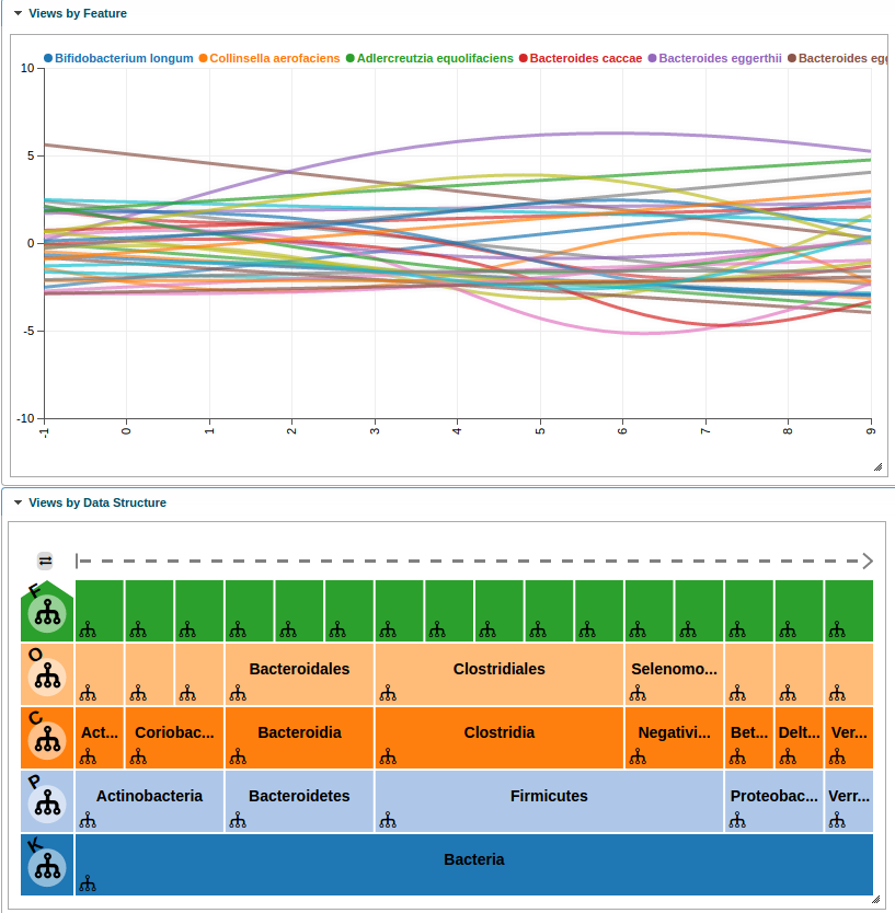
Spline metavizr
Close Metavizr and end session
To close the connection with metaviz and the R session, we use the stop_app function.
app$stop_app()SessionInfo
sessionInfo()## R version 3.3.1 (2016-06-21)
## Platform: x86_64-pc-linux-gnu (64-bit)
## Running under: Ubuntu 14.04.5 LTS
##
## locale:
## [1] LC_CTYPE=en_US.UTF-8 LC_NUMERIC=C
## [3] LC_TIME=en_US.UTF-8 LC_COLLATE=en_US.UTF-8
## [5] LC_MONETARY=en_US.UTF-8 LC_MESSAGES=en_US.UTF-8
## [7] LC_PAPER=en_US.UTF-8 LC_NAME=C
## [9] LC_ADDRESS=C LC_TELEPHONE=C
## [11] LC_MEASUREMENT=en_US.UTF-8 LC_IDENTIFICATION=C
##
## attached base packages:
## [1] parallel stats graphics grDevices utils datasets methods
## [8] base
##
## other attached packages:
## [1] metavizr_0.99.5 etec16s_1.0.0 msd16s_0.106.0
## [4] metagenomeSeq_1.17.0 RColorBrewer_1.1-2 glmnet_2.0-5
## [7] foreach_1.4.3 Matrix_1.2-7.1 limma_3.28.21
## [10] Biobase_2.32.0 BiocGenerics_0.18.0 devtools_1.12.0.9000
##
## loaded via a namespace (and not attached):
## [1] nlme_3.1-128 bitops_1.0-6
## [3] matrixStats_0.51.0 phyloseq_1.16.2
## [5] httr_1.2.1 rprojroot_1.2
## [7] GenomeInfoDb_1.8.7 highlight_0.4.7
## [9] tools_3.3.1 backports_1.0.5
## [11] epivizr_2.5.1 vegan_2.4-1
## [13] R6_2.2.0 KernSmooth_2.23-15
## [15] mgcv_1.8-16 colorspace_1.3-2
## [17] DBI_0.5-1 lazyeval_0.2.0
## [19] permute_0.9-4 ade4_1.7-5
## [21] withr_1.0.2 curl_2.3
## [23] git2r_0.18.0 graph_1.50.0
## [25] xml2_1.1.1 desc_1.1.0
## [27] rtracklayer_1.32.2 scales_0.4.1
## [29] caTools_1.17.1 RBGL_1.48.1
## [31] pkgdown_0.1.0.9000 commonmark_1.1
## [33] stringr_1.1.0 digest_0.6.12
## [35] Rsamtools_1.24.0 epivizrStandalone_1.1.8
## [37] rmarkdown_1.3.9002 XVector_0.12.1
## [39] epivizrServer_1.3.1 htmltools_0.3.5
## [41] RSQLite_1.1-2 BiocInstaller_1.22.3
## [43] jsonlite_1.2 BiocParallel_1.6.6
## [45] gtools_3.5.0 RCurl_1.95-4.8
## [47] magrittr_1.5 biomformat_1.0.2
## [49] munsell_0.4.3 Rcpp_0.12.9
## [51] S4Vectors_0.10.3 ape_4.0
## [53] stringi_1.1.2 whisker_0.3-2
## [55] yaml_2.1.14 MASS_7.3-45
## [57] SummarizedExperiment_1.2.3 zlibbioc_1.18.0
## [59] rhdf5_2.16.0 pkgbuild_0.0.0.9000
## [61] gplots_3.0.1 plyr_1.8.4
## [63] grid_3.3.1 gdata_2.17.0
## [65] crayon_1.3.2 lattice_0.20-34
## [67] splines_3.3.1 Biostrings_2.40.2
## [69] multtest_2.28.0 GenomicFeatures_1.24.5
## [71] RNeo4j_1.6.4 knitr_1.15.1
## [73] igraph_1.0.1 GenomicRanges_1.24.3
## [75] rjson_0.2.15 reshape2_1.4.2
## [77] codetools_0.2-15 biomaRt_2.28.0
## [79] stats4_3.3.1 pkgload_0.0.0.9000
## [81] XML_3.98-1.5 evaluate_0.10
## [83] data.table_1.10.0 httpuv_1.3.3
## [85] testthat_1.0.2 gtable_0.2.0
## [87] purrr_0.2.2 assertthat_0.1
## [89] ggplot2_2.2.1 mime_0.5
## [91] roxygen2_6.0.0 survival_2.40-1
## [93] tibble_1.2 OrganismDbi_1.14.1
## [95] iterators_1.0.8 epivizrData_1.3.0
## [97] GenomicAlignments_1.8.4 AnnotationDbi_1.34.4
## [99] memoise_1.0.0 IRanges_2.6.1
## [101] cluster_2.0.5 gss_2.1-6References:
[1] Pop, M., Walker, A.W., Paulson, J., Lindsay, B., Antonio, M., Hossain, M.A., Oundo, J., Tamboura, B., Mai, V., Astrovskaya, I. and Bravo, H.C., 2014. Diarrhea in young children from low-income countries leads to large-scale alterations in intestinal microbiota composition. Genome biology, 15(6), p.1.
[2] Pop, M., Paulson, J.N., Chakraborty, S., Astrovskaya, I., Lindsay, B.R., Li, S., Bravo, H.C., Harro, C., Parkhill, J., Walker, A.W. and Walker, R.I., 2016. Individual-specific changes in the human gut microbiota after challenge with enterotoxigenic Escherichia coli and subsequent ciprofloxacin treatment. BMC genomics, 17(1), p.1.
[3] Paulson J.N., Talukder H., and Bravo H.C, Longitudinal differential abundance analysis of microbial marker-gene surveys using smoothing splines. In Submission.